This is a Python lab exercise that has been converted from Jupyter to an MD-format post to illustrate the interaction between derivative and inverse functions.
Understanding Derivative-Based Methods: Imagine you’re driving a car and want to know how fast you’re going at any moment. The speedometer tells you your speed, which is the rate of change of your position with respect to time. In calculus, this idea is captured by the derivative. A derivative measures how a function changes as its input changes — it’s like the speedometer for mathematical functions. Derivative-based methods use this concept to find slopes of curves, rates of change, and to solve problems involving optimization (finding maximum or minimum values).
Visualization of Derivatives: Think of a curve on a graph representing a function, like a winding road. At any point on this road, the derivative tells you the slope of the road — whether it’s going uphill, downhill, or flat. Visualizing this slope as a tangent line touching the curve at just one point helps you see how the function behaves locally. For example, where the tangent line is flat (slope zero), the function might have a peak or a valley, indicating a maximum or minimum.
Visualizing the derivative of an inverse function involves understanding the relationship between a function and its inverse, especially how their slopes relate.
Key idea:
-
If is invertible, its inverse satisfies:
Which slightly more standart formulation is:
This means the slope of the inverse function at a point is the reciprocal of the slope of the original function at the corresponding point.
To visualize this in Python:
- Plot the original function and its inverse .
- Plot tangent lines at corresponding points on both curves.
- Show that the slopes of these tangent lines are reciprocals.
import numpy as np
import matplotlib.pyplot as plt

# Original function: f(x) = x^2, restricted to x >= 0
def f(x):
    return x**2

# Derivative of f
def df(x):
    return 2 * x

# Inverse function: f^{-1}(y) = sqrt(y)
def f_inv(y):
    return np.sqrt(y)

# Derivative of inverse function using reciprocal rule
def df_inv(y):
    x = f_inv(y)
    return 1 / df(x)

# Choose a point to visualize tangent lines
x0 = 2
y0 = f(x0)

# Points for plotting
x_vals = np.linspace(0, 4, 400)
y_vals = f(x_vals)
y_inv_vals = np.linspace(0, 16, 400)
x_inv_vals = f_inv(y_inv_vals)

plt.figure(figsize=(10, 6))

# Plot original function and inverse
plt.plot(x_vals, y_vals, label='f(x) = x^2')
plt.plot(x_inv_vals, y_inv_vals, label='f⁻¹(y) = sqrt(y)')

# Tangent line at (x0, y0) on f
slope_f = df(x0)
tangent_f_x = np.linspace(x0 - 1, x0 + 1, 10)
tangent_f_y = slope_f * (tangent_f_x - x0) + y0
plt.plot(tangent_f_x, tangent_f_y, 'r--', label='Tangent to f at x=2')

# Tangent line at (y0, x0) on f_inv
slope_f_inv = df_inv(y0)
tangent_f_inv_y = np.linspace(y0 - 4, y0 + 4, 10)
tangent_f_inv_x = slope_f_inv * (tangent_f_inv_y - y0) + x0
plt.plot(tangent_f_inv_x, tangent_f_inv_y, 'g--', label='Tangent to f⁻¹ at y=4')

plt.xlabel('x or f⁻¹(y)')
plt.ylabel('f(x) or y')
plt.title('Function and Inverse with Tangent Lines')
plt.legend()
plt.grid(True)
plt.show()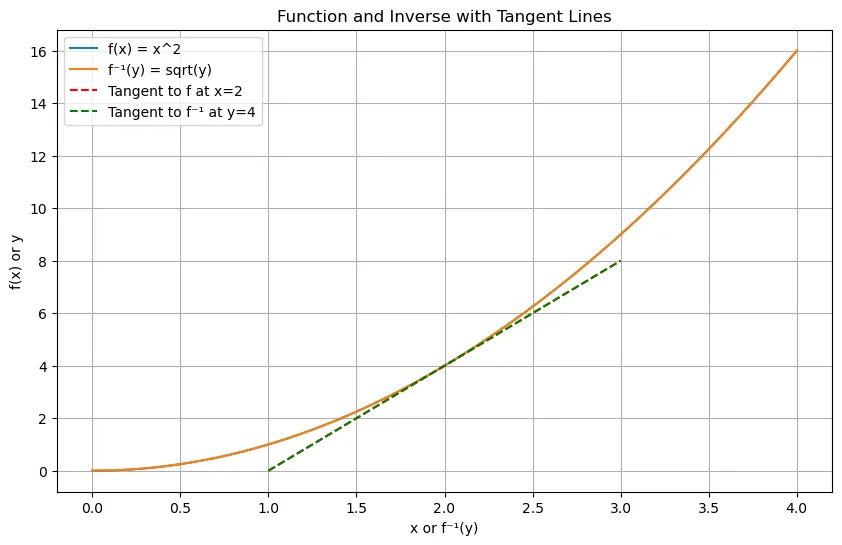
This plot shows:
- The function (right branch),
- Its inverse ,
- Tangent lines at corresponding points,
- The slopes of these tangent lines are reciprocals.
How does the reciprocal relationship of slopes affect function behavior?
The reciprocal relationship of slopes between a function and its inverse has important implications for their behavior:
- When the original function’s slope is steep (large magnitude), the inverse function’s slope is shallow (small magnitude), because the inverse slope is the reciprocal.
- Conversely, when the original function’s slope is close to zero (flat), the inverse function’s slope becomes very large (steep).
- This means that near points where the original function changes slowly, the inverse changes rapidly, and vice versa.
- It also implies that the inverse function “flips” the rate of change, reflecting the input-output roles.
In practical terms, this affects how sensitive the inverse function is to changes in its input compared to the original function.